iDanae Chair quarterly newsletter: Machine Learning Algorithms

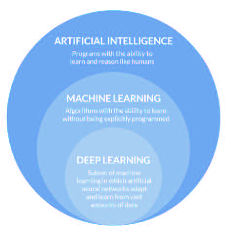
These three terms are often used interchangeably as synonyms. Conceptually, however, Artificial Intelligence can be considered the broadest field in which the other disciplines can be included (see Figure 1).

More precisely, Artificial Intelligence is an area of computing that relates to how to make machines perform human-like tasks, i.e. trying to simulate intelligent behaviour. Machine Learning can be considered a subfield of artificial intelligence that allows computers to learn from data without being explicitly programmed for it, providing an intelligent system with the ability to perform a certain task. Thus, Machine Learning can be defined as a set of methods that can automatically detect patterns in data, and use them to predict future data, or to perform other kinds of decision making under uncertainty.

Finally, el Deep Learning also allows computers to learn from data, based on the use of complex multi-layered neural networks, where the level of abstraction gradually increases through non-linear transformations of the data. Within this framework, this newsletter focuses on the discipline of Machine Learning.

The rise of this area entails multiple discussions around some main challenges: the ability to model causality,the business approach for using Artificial Intelligence from an ethical and an organizational point of view, etc. There are also other technical elements that need to be considered, such as the quality of the data, its insufficiency or not representativeness, or the necessary computational capacity, among others. In addition to these elements, and as a basis of the discipline, there is also the need to understand the learning algorithms on which this field of knowledge is based. Therefore, this newsletter aims to give an overview of the most commonly used Machine Learning algorithms, in order to provide a knowledge base for the correct use of the different algorithms.

Types of algorithms

Within Machine Learning algorithms, there are several categorisations according to different criteria: the supervision during training, the possibility of carrying out incremental learning, the way for generalising the results, etc. It should be noted that these classifications are not necessarily static, and in some cases new concepts have been incorporated as a result of the appearance of new techniques whose nature did not fit within any of the existing categories.

First of all, it is necessary to make a distinction, based on functionality, between descriptive and predictive algorithms, which is a widespread categorisation within the field of data mining. A descriptive algorithm aims to describe the population by exploring the properties and characteristics of the data, while a predictive algorithm aims to make predictions about unknown future events from historical data. In turn, each category can be broken down into several subcategories, allowing a more detailed classification of algorithms. In the case of descriptive algorithms, the following subcategories can be considered: (1) clustering, (2) summarization, (3) association rules, and (4) sequence discovery; in the case of predictive algorithms, the two main categories are (1) classification and (2) value estimation.

However, nowadays it is more common to use a classification based on the type of available data, i.e. according to whether labelled or unlabelled data are available. Four categories can be distinguished:

Supervised Learning: Supervised learning algorithms attempt to model the relationships between the input data and the target variable, so that values of the target variable can be predicted for new data based on relationships learned from labelled historical data. To infer these relationships, the training sets used must include the values of the target variable, commonly called "labels".

There are two main types of supervised learning:

• Classification: its goal is to predict the class to which a specific sample belongs, e.g. to determine if an email is spam or not. The target variable is discrete (generally, it is a finite set of classes).
• Value estimation: its goal is to predict a numerical value, e.g. the selling price of a house. Therefore, the target variable is usually continuous (although the final prediction may be a discrete set of values represented by an indicator, such as a group mean).

Unsupervised Learning: Unsupervised learning algorithms allow inferring patterns or relationships in unlabelled data sets. In contrast to supervised learning, a target value is not predicted (no labels are available), but rather the data is explored and inferences are made to discover hidden structures in the data.

 
The following types of unsupervised learning algorithms can be highlighted (non-exhaustive list):

• Clustering: its goal is to find groups or clusters of similar individuals or variables existing in the data, e.g. homogeneous groups of customers to carry out market segmentation.
• Association rule learning: its goal is to discover relationships between variables, extracting rules and patterns from the data; e.g. to determine consumption patterns.
• Other algorithms: multiple algorithms do not fall into the above categories; some of them are frequently used in processes such as dimensionality reduction or anomaly detection algorithms, which are commonly used in data pre-processing. Due to their use in some modeling phases, these algorithms will not be discussed in this newsletter.

Semi-supervised learning: this is a hybrid approach between supervised and unsupervised learning. In this case, the training data are partially labelled sets, where a few examples are labelled and a large number of examples are unlabelled. The goal of these algorithms is to make effective use of all available data, not just the labelled ones. These models are typically used when labelling the data may be too time-consuming, too expensive, or not available for part of the sample.

Reinforcement learning: it encompasses problems in which an agent learns to operate in an environment through a process of feedback (i.e., trial and error). The goal of these algorithms is to use the information obtained from interaction with the environment to perform those actions that maximise the reward or minimise the risk; the iterative learning consists of exploring different possibilities. There is no training data set, but rather a goal to be achieved by the agent, a set of actions it can perform, and feedback on its performance.
 

Under this categorisation, the following sections will delve into the main algorithms corresponding to the categories of supervised and unsupervised learning, as these are currently the most commonly used.

Supervised and unsupervised algorithms

In this section, a brief overview of the main supervised and unsupervised learning algorithms that can be used to solve a problem is provided. The choice of model will depend on both the type of data and the type of task to be performed, and also the model validation is essential.

Supervised learning

As discussed in the previous section, supervised learning algorithms attempt to model the relationships between the input data and the target variable. Depending on whether the target variable is discrete or continuous, this is a classification or value estimation problem, respectively.

Model training

In general terms, a supervised learning algorithm is trained from pattern models, examining a set of examples and trying to find the parameters that minimise or maximise an objective function, commonly referred to as a loss function. In this way, the parameters or weights of the model are iteratively adjusted to approximate the optimum of the objective function.

In more detail, the loss function is used as a measure of how well the model performs in terms of its predictive power. There are several factors involved in the choice of this function, but there is a clear differentiation according to the type of task to be performed, value estimation or classification problems.

Among the loss functions for value estimation, the mean square error (MSE) is one of the most widely used. It is calculated as the average of the quadratic difference between actual observations and predictions, and is represented by the following equation:

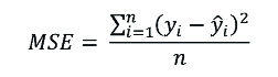
Thus, this function measures the average magnitude of the error, regardless of its direction. 

For classification problems, the cross-entropy is one of the most commonly used loss functions. It measures the performance of models whose output is a probability value between 0 and 1. Mathematically, it can be formulated by the equation:

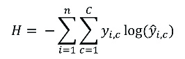
The value of this function will increase as the predicted probability differs from the actual label, strongly penalising predictions that are certain, but wrong.

Model performance

Performance is a critical factor in the choice of a model. A good classification model should not only fit the data it has been trained on, but should also perform well on new instances never seen before. This second part refers to the generalisation capacity of the model. Therefore, a distinction is made between training error (calculated on the data set on which the model was trained) and validation or test error (calculated on an independent data set, which was not used in the training). 

Therefore, it is said that the model has a good performance if the validation error remains bounded, and in the same order of magnitude as the training error. Consequently, the validation error is a good way to measure model performance. For its estimation, due to data limitations, it is common to use the hold-out method, whereby the data set is divided into training and test subsets. However, another more robust alternative for estimating this error is cross-validation, a method by which the data set is divided into k groups, k-1 groups are used for training and one for testing the model.

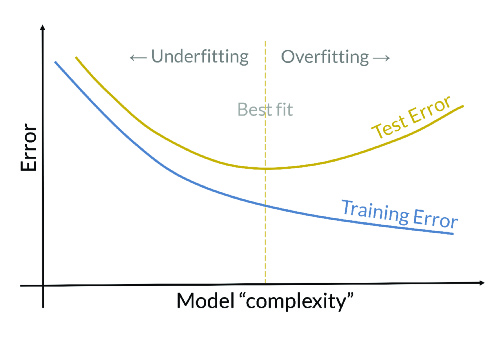
If the generalisation error were significantly larger than the training error, the model would be overfitting the training data, which implies that the model is not able to generalise well on new data. This situation is called overfitting, and its probability of occurrence increases as the complexity of the model increases. Therefore, according to Ockham's razor principle, between two models with the same validation error, the simplest is to be selected. However, if the training error were too high, the model would not be able to model the training data, and therefore not be able to generalise to new data, which is called underfitting. The next figure shows both situations.

However, despite the use of a common methodology, the way in which predictions will be evaluated will differ depending on whether it is a classification or a value estimation problem. The main measures used in each category are set out below. 

Clasification

• Confusion matrix n x n23, where the rows refer to the actual classes and the columns to the predicted classes, explicitly showing the number of instances of each class predicted correctly and the number of instances where one class has been confused with the other.
• Accuracy: proportion of correct predictions made by the model.
• Precision: fraction of predicted correctly classified, i.e. how many of those predicted are really of the predicted category.
• Recall: fraction of correctly classified examples out of the total number of examples in a given class.
• F1-Score: harmonic mean of the measures Precision and Recall.

Value estimation

• Mean square error: average of the squared difference between actual observations and predictions.
• Root mean square error: square root of the average of the squared differences between actual observations and predictions.
• R2: proportion of variability explained by the model.

Finally, it should be noted that achieving good performance does not depend only on the chosen algorithm. Without pre-processing of the data, accurate results might not be obtained, regardless of the algorithm.

Main algorithms

Once both training and validation of a model have been addressed, the main algorithms under the supervised learning category are presented. No differentiation is made between classification and value estimation algorithms because some of them can be used for both tasks.

 
Linear regression

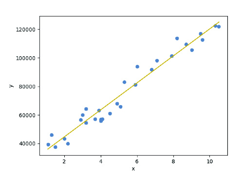
It is a linear approach to modelling the relationship between a continuous response variable (dependent variable) and one or more explanatory variables (independent variables). The case of one explanatory variable is called simple linear regression, represented mathematically by the equation:

Y=a+bX

Where X is the independent variable and Y is the dependent variable. The slope is b and the intercept is a, being these the coefficients of the model to be estimated, usually adjusted by the least-squares method. An example of simple linear regression can be seen in the next figure.

This model is usually a good baseline for estimation value problems. However, it is important to corroborate the fulfilment of the model's hypotheses: (1) linearity, (2) homoscedasticity, (3) independence and (4) normality.

Logistic Regression

It is a statistical method used in classification problems, predicting the probability of occurrence of different possible outcomes. Specifically, this algorithm looks for a hyperplane that is capable of linearly separating classes.

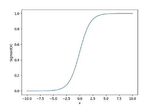
Unlike linear regression, the dependent variable is categorical, i.e. it takes a limited number of values. When this variable has only two possible values, it is called simple logistic regression, predicting the probability of occurrence of that event. Mathematically, it is formulated by the equation:

y= σ(a+bX)

Where σ is the sigmoid function, which is responsible for assigning probabilities to the predicted values.

As a consequence of its simple formulation, this model is considered a good baseline to use in classification problems.

K-nearest neighbours (k-nn)

It is a nonparametric lazy learning algorithm that can be used to solve both classification and value estimation problems.

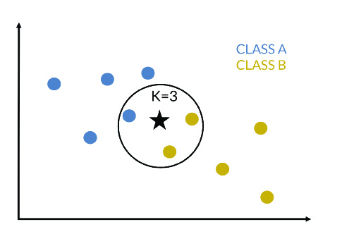
More precisely, given a new instance to be classified, the distances of this point from the instances that make up the training set are calculated, the nearest k-instances are selected and the average of the numerical labels is calculated (in a regression problem) or the most frequent class is selected (in a classification problem). In Figure 6, an example of 3-nn is presented, where the new instance will belong to class B.

Its widespread use is due to its good performance, simplicity and versatility; however, its disadvantages must also be taken into account: (1) difficulty in determining the optimal k, (2) need to store the training set, and (3) execution time proportional to data size.

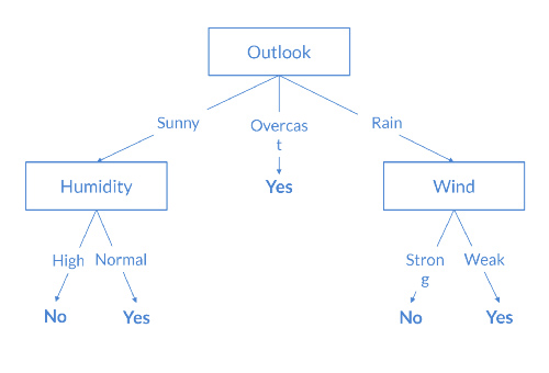
Decision trees

This algorithm is based on the "divide and conquer" strategy. It is used for both classification and value estimation problems, being its objective to predict the value of the target variable from simple decision rules inferred from the data. In other words, this algorithm subdivides the feature space into regions, mapping each of the final regions to a value of the target variable. Thus, it is a simple and interpretable model, which provides an explanation of the results inferred by the model. In the next figure, a decision tree used in a binary classification task can be visualised.

Naive Bayes

It is a classification algorithm based on Bayes' theorem.This classifier assumes that the variables are independent and that each variable contributes equivalently to the outcome. However, these assumptions are not usually satisfied in real problems; the independence assumption is rarely satisfied, but even so, this algorithm usually works well in practice.

Mathematically, according to Bayes' theorem, the following relationship is established:

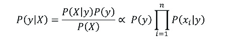
Where y is the class and  X=(x1,x2,…,xn) is the set of features. Thus, the predicted class will be that with the highest probability.

It is a simple and robust technique, which tolerates missing values satisfactorily. However, if a categorical variable has a category that is not observed in the training set, the model will assign a probability of 0 and no prediction can be made.

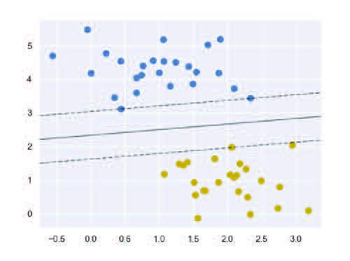
Support Vector Machine

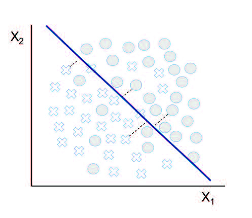
This popular algorithm can be used for both classification and value estimation tasks, although it is more widely used for classification tasks. Its goal is to find a hyperplane, in an N-dimensional space, that separates classes of points by transforming the explanatory variables using kernel functions. These functions are used to map non-linearly separable functions into linearly separable functions of higher dimension.

More specifically, a hyperplane that maximises the distance between the data points of the classes (called the margin) has to be found in a higher dimensional space compared to the space of the data. This way, a larger margin of confidence is tried to be achieved for future predictions. In the next figure, an example can be visualised in which both the hyperplane that best separates the data and the margin are represented.

In order to use this algorithm, it should be considered that the training process can take a long time if a large dataset is used.

Neural networks

The increase in computational capacity, as well as the increase in the volume and typology of data, has led to extensive development in the field of neural networks, which has led to a rise in the Deep Learning discipline.

In this context, in which the processing of unstructured data (text, audio, images and video) has become an important source of information, the areas of Natural Language Processing and Computer Vision have advanced rapidly.

However, due to the large number of existing types of neural networks and their complexity, this type of algorithms is not addressed in this newsletter.

Learning Improvement Techniques: Ensemble Methods

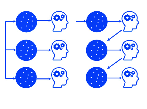
Ensemble methods are based on the combination of multiple models in order to obtain better results using joint knowledge and can be used for both classification and estimation value tasks. There are two main techniques:
 

• Bagging: The models are trained in parallel and the combination of the predictions is used as the final prediction.
• Boosting: The models are trained sequentially so that each model tries to correct the errors of the previous model.

Some of the most commonly used ensemble methods are briefly described below:

• Random Forest: This bagging algorithm creates several decision trees in parallel and merges them by combining their predictions to obtain more accurate and stable predictions.
• Gradient Boosting: As the name suggests, this is a boosting algorithm. This method sequentially combines a series of trees, so that each tree focuses on correcting the error of the previous tree. More precisely, this is done by modelling the prediction error of the previous decision tree. In particular, a specific implementation of this algorithm is XGBoost, which seeks to improve the speed of execution and performance of the model.
• AdaBoost: This algorithm is similar to the previous one, but differs in the way in which each tree corrects the error of the previous tree. In this case, in each iteration the weightings of the observations are updated according to the errors made, so that a greater weight is assigned to those observations that the model has not been able to predict correctly.

Unsupervised Learning

Unsupervised learning algorithms aim to discover hidden patterns in unlabelled data. The lack of these labels means the absence of a benchmark against which to evaluate the quality of the model, which increases the complexity of model validation. In this section, the examples presented fall into the categories described above.

Clustering

These algorithms, which aim to discover natural groupings in the data, are based on the hypothesis that observations belonging to the same group should have similar characteristics; and, on the contrary, observations belonging to different groups should have different characteristics. This type of algorithm aims to group the data in such a way that the instances of a group are similar to each other (minimising the intra-group distance) and different from other groups (maximising the inter-group distance).

There is a wide variety of clustering algorithms, each of them offering a different approach to perform the task. The main categories into which these algorithms are grouped are the following:

• Partitive clustering: Partitions are generated according to a similarity measure. E.g. k-means, pam.
• Hierarchical clustering: It seeks to construct a hierarchy of clusters, called dendogram. There are two clearly differentiated approaches: 
  • Agglomerative (bottom-up approach): each observation forms its own cluster initially, and they are merged according to a similarity condition. The algorithm usually stops when a certain criterion is satisfied, thus generating several clusters. E.g. agnes.
  • Divisive (top-down approach): all observations are initially included in a single cluster and divisions are performed recursively. The algorithm usually stops when a certain criterion is satisfied, thus generating several clusters. E.g. diana.
• Fuzzy clustering: The assignment of instances to any of the clusters is not fixed, and an instance may belong to more than one cluster. E.g. fanny, daisy.
• Density based clustering: Clusters are created according to the density of data points. E.g. DBSCAN, OPTICS, meanshift.
• Others: based on graphs (spectral), or based on probabilistic models (mixture models), among others.
   

The choice of which algorithm to use is complex and not immediate, and requires experimentation on the dataset. Therefore, there is no best algorithm, but the suitability of one or the other will depend on the inherent distribution of the data.

In any case, it is important to quantify the performance of the clustering obtained. In general, one can distinguish between extrinsic measures, which require knowledge of the true labels, and intrinsic measures, which measure the goodness of results without considering external information. In accordance with the definition of unsupervised learning, under which no labelled data are available, the focus in this newsletter is on intrinsic validation, and it is common to distinguish between cohesion and separation measures. Specifically, cohesion measures determine the degree of proximity of the points that make up a cluster, while separation measures determine the degree of separation of clusters. Some of the most commonly used intrinsic measures are the following:

• Silhouette coefficient: calculated for each instance of the dataset as where a measures cohesion as the average distance from that instance to the rest of the instances in that cluster and b measures separation as the average distance from that instance to the set of instances that builds the nearest cluster. The calculation of this measure at cluster level is calculated as the average of this coefficient for all its instances. This coefficient is bounded to the interval [-1, 1] where a higher value will be indicative of better defined clusters.

• Davies-Bouldin Index: is calculated as the average similarity of each cluster to its most similar cluster. The lower the value, the better the partition, being 0 the minimum value of this index.
• Dunn Index: is defined as the ratio between the minimum inter-cluster distance and the maximum intra-cluster distance. The higher the value, the better the clustering.

Finally, some of the most commonly used clustering algorithms are presented:
 

• K-means: It is probably the best-known and most widely used clustering algorithm. By specifying a number of clusters a priori, the algorithm allows assigning each observation to the nearest centroid. In particular, k centroids are selected at random, and through an iterative process, each point is assigned to its nearest centroid, updating at each step the value of the centroids.
• DBSCAN (density-based spatial clustering of applications with noise): It is a density-based algorithm, i.e., it assumes the existence of a cluster when it identifies a dense region, which allows detecting as outliers those points that do not exceed an established density threshold. In this way, this algorithm is based on detecting points with sufficient density and building clusters around them, adding points close to it. To do this, it is necessary to specify the maximum distance for two points to be considered neighbours and the minimum number of points to form a cluster.

The next figure shows a comparison of the results obtained with these two methods on different datasets.

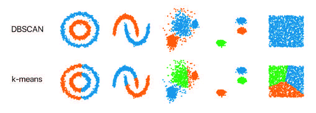
The following advantages of the DBSCAN algorithm over the k-means algorithm can be highlighted: (1) it can find clusters with arbitrary geometric shapes; (2) it has the ability to detect outliers; (3) it is not necessary to specify the number of clusters; and (4) consistency in its results in different runs. On the other hand, the performance of the k-means algorithm is slightly better due to its simplicity.

Association rule learning

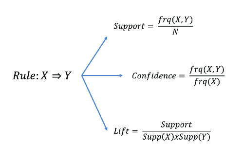
It covers rule-based methods that are used to uncover hidden relationships in data. More precisely, an association rule consists of an antecedent (if) and a consequent (then), reflecting a co-occurrence relationship, i.e. the consequent is something that occurs when an antecedent occurs.

 
{Precedent}→ {Consequent}

It is worth mentioning that this type of rule extraction from data has two problems: (1) discovering rules from large data sets can be computationally expensive and (2) some of the extracted patterns may occur by chance. To help deal with these problems, several metrics determine the strength of the association: (1) support: frequency with which an element or set of elements appears in the dataset; (2) confidence: frequency with which the rule is true; and (3) lift: increase in the probability of the consequent occurring when the antecedent has already occurred.

• A priori algorithm: it was the first algorithm proposed for this type of problems. Conceptually, it is based on generating a set of frequent items (items whose support is greater than a set threshold) and generating association rules from this reduced set, selecting those with a high level of confidence.
• ECLAT (Equivalence Class Transformation) algorithm: this algorithm uses a depth-first search to find the most frequent items set, which makes it a faster algorithm than the a priori algorithm.

Most frequent algorithms

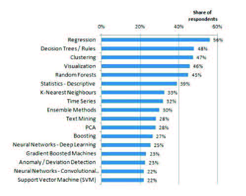
Once the main Machine Learning algorithms have been presented, it is interesting to visualise which are the most used algorithms in actual applications. Next figure presents the results obtained according to the survey conducted by KDnuggets in the period 2018/2019. Under this study, the three most used methods are regression, decision trees and clustering algorithms, being simple and interpretable models.

In addition, according to to another survey conducted in 2017, an increase in the use of Deep Learning techniques (generative adversarial networks, recurrent neural networks, convolutional networks, etc.) can be observed, accompanied by a decrease in the use of algorithms such as SVM and association rules.

How to put these algorithms into practice?

After presenting the main Machine Learning algorithms, it is necessary to discuss how they can be used from a practical point of view to solve a given task.

A frequent question is which programming language to use for ML tasks, given the great diversity of available languages. There is no best or preferred programming language, although there are some languages that are more appropriate than others depending on the problem to be addressed. The following are some of the most popular ones:

• Python: it has become the favourite programming language in the Machine Learning field55 thanks to: (1) its wide ecosystem of libraries (scikit-learn, numpy, pandas, keras, tensorflow, etc.), (2) the readability of the code thanks to its simple syntax and (3) its multi-paradigm and flexible nature.
• R: is another popular choice, being a statistics-oriented language, which provides a wide range of packages. Specifically, this language focuses on statistical modelling and analysis. Among its main drawbacks are its learning curve and its speed.
• Julia: is a high-level programming language that was designed for high-performance numerical analysis and computational science. Julia attempts to make up for the shortcomings of Python and R in terms of performance, while maintaining rapid development. However, it has not managed to achieve the popularity of Python or R. 

Moreover, all this has been generalised by the availability of these languages both in laboratory environments and in production environments, either on-premise or in the Cloud. These environments integrate recent technological breakthroughs (such as the incorporation of GPUs with extensions for deep learning, or tensor processing units or TPUs), which dramatically increases both the computing power and energy efficiency of computational systems. All of this makes it possible to take advantage of the available technological infrastructure, at an ever-decreasing cost. 

The "Machine Learning Algorithms​" newsletter is now available for download on the Chair's website in both in spanish and english​.​​