iDanae Chair newsletter: Deep Learning

In the field of Artificial Intelligence, the discipline of Machine Learning tries to solve complex problems through the application of techniques and algorithms that allow information to be extracted from large volumes of data, which have been generated by the real systems that are to be analysed. Many of these problems can be solved using relatively simple algorithms. However, there are many complex cases where advanced techniques have to be applied, for example due to the difficulty of the task to be performed or the complexity of the function to be represented. This is the case for computer vision, audio processing, natural language processing, complex search algorithms, etc. 

In these cases, a set of techniques have proven to be useful in solving these or other tasks, and which are grouped under the name of Deep Learning. This discipline can be defined as "a solution that allows the computer to learn from experience in terms of a hierarchy of concepts, where each concept is defined through its relationship with simpler concepts. […] The graph that would represent how these concepts are built upon each other is deep, with many layers". 

In general, Deep Learning architectures are represented through the so-called neural networks: representations where input information is combined in multiple layers through weights or parameters and specific functions to obtain a given result. Deep Learning can therefore be understood as an evolution of some specific machine learning techniques. Although Deep Learning techniques began to be established in the second half of the 20th century, their development has been boosted in recent decades due to the improved performance of the solutions obtained, the greater availability of data used for training (derived from better capture processes, sensorisation, etc.), and the greater technological capacity to exploit this data and train structures with an enormous amount of parameters.

This discipline draws on various fields of knowledge to obtain neural networks: statistical methods (for the analysis of the input data on which the training will be performed, the detection of possible biases and limitations, or the understanding of the results obtained), linear algebra (applied in the representation of the architecture of coefficients or in the implementation of some algorithms), calculus techniques (since the parameters are obtained as a result of the search for the minimum of error functions), or computer science (which allows the programming of complex processes through the use of libraries and algorithms already implemented that allow a simple and optimised use).

The use of neural networks has a number of advantages in terms of applicability and computation
 

• Neural networks are flexible and can be used for both regression (continuous) and classification (discrete) problems. Any numerical data can be used in the model, as the neural network uses approximation functions.
• Neural networks work well in modelling non-linear data with a large number of inputs, e.g. images.
• Once trained, the networks can make predictions fairly quickly.
• Neural networks can be trained with any number of inputs and layers, allowing for a theoretically unlimited representation capacity (i.e. they are universal approximators of functions).
• Neural networks work well with large data sets and with good density in probability space: they are able to exploit much of the available information given the parametric capability.

However, several risks associated with the use of neural networks and their implementation in organisations need to be considered. Among others, the need for large volumes of quality data for training multiple parameters, the possible over-fitting to the data that can lead to loss of generalization capacity, or the difficulty of interpreting the model or its results, given the complexity of the relationships that are obtained. These challenges are explored in the last section of this paper.

There are multiple types of neural networks, each of which can be applied to different problems: multilayer perceptron networks, autoencoders, convolutional networks, recurrent networks, etc. In the following sections, the main concepts of this discipline are reviewed, different training processes for these models are presented, and different architectures that can be used to solve problems are analysed.

Neural Networks

Concept and components

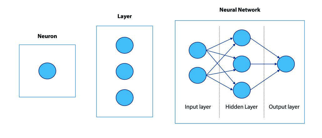
Conceptually, the models and algorithms under study in Deep Learning, the so-called artificial neural networks, can be compared to networks of biological neurons when understood as sets of elements (neurons) that are connected to each other, forming a network structure. This structure allows each neuron to communicate and "transmit information" through its connections with other neurons, giving rise to complex behaviours that can be interpreted as intelligent.

An artificial neural network can therefore be conceptualised as a set of variables that are combined through weights and act as inputs to the different neurons. A mathematical function, called an activation function, is applied in each neuron and produces an output. This output can in turn work as a new input variable for another neuron, thus combining the information in different layers until a final solution is obtained.

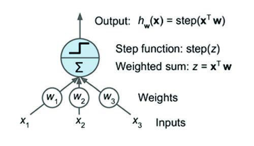
The simplest model on which modern artificial neurons are based is known as the McCulloch-Pitts neural model
(McCulloch, Pitts 1943) . This model is based on the premise that part of the biological processes can be mimicked by a function that receives a list of input signals weighted by parameters, and outputs some kind of signal if the sum of these weighted inputs reaches a certain threshold.

This model was the first to introduce the concept of an artificial neuron and has only two types of inputs, "excitatory" and "inhibitory". Excitatory inputs have positive magnitude weights and inhibitory inputs have negative magnitude weights. The inputs to the McCulloch-Pitts neuron can be either 0 or 1 and use a threshold function as an activation function where the output signal is 1 if the input is greater than or equal to a given threshold value, and 0 otherwise. However, this does not allow for fitting the full intermediate range of behaviours which facilitates fitting and with desirable mathematical properties, such as differentiability, essential to enable training.

A more current approach is to change certain aspects of the McCulloch-Pitts model, to allow the connection of multiple layers without losing the desired mathematical properties to train them. Instead of working as a switch that can only receive and output binary signals, modern artificial neurons use continuous values with continuous activation functions. Thus, neurons under this model are functions of the form y=f(x,w,b), where x represents the input variables, w represents the weights or parameters, b represents the bias (constant additive values, y represents an additional input in the next layer that will always have the value of 1), and f is the activation function.

To keep the range of neuron values bounded, activation functions are used. These functions add non-linearity to the output functions they model, allowing neural networks to construct complex multidimensional surfaces capable of fitting non-linear problems (in fact, a neural network without an activation function is essentially a linear regression model).

Extending the single neuron expression to the case of multiple layers transmitting information between them, a structure is obtained where the outputs of one layer (represented by y) correspond to the inputs of the next (represented by x), which are transformed by the weights and biases of each neuron. In this way the set of weights can be represented as a matrix n x m (m neurons of the layer by n information entries corresponding to the n neurons of the previous layer).

NN training

In essence, training a neural network consists of finding the parameters that minimise the function that measures the prediction error on a set of data: the cost function. To do this, different optimisation algorithms and techniques are applied, as described below.

The cost function

The cost function is defined as an aggregation, usually by the mean, of loss functions that measure the errors made for each sample: A cost function, noted by J(w,b,X,ytrue), ), is a measure of the error between the value predicted by the model and the actual value. This function will be the guideline used to monitor the performance of the network and adjust its parameters automatically and iteratively by the optimisation algorithm. 

A multitude of loss functions can be defined depending on the type of problem and the characteristics of the dependent variable, although usually maximum-likelihood estimators are used (such as the LogLoss, known as Binary Crossentropy for binary problems, Categorical Crossentropy for multi-class problems or other loss functions such as the Mean Squared Error [MSE] for regression problems). In any case, these functions can be any error measure that has good differentiability properties, essential to train the model automatically.

Optimisation algorithms: Backpropagation

In Deep Learning, contexts, optimisation is the process of changing the parameters of the model to improve its performance. In other words, it is the process of finding the best weights in the predefined hypothesis space to obtain the best possible performance. There are no analytical methods for training neural networks (except in the simplest cases composed of a single neuron), so numerical optimisation algorithms are used to tackle the problem.

To train the network, the error propagation starts at the output layer until it reaches the input layer via the hidden layers (if any). This process of error propagation is called backpropagation.

The backpropagation algorithm aims to determine the contribution of each parameter to the cost function. To do this, the chain rule of differential calculus is used, which allows each of these contributions to be determined as a product of derivatives. The derivatives of each parameter in each layer must be pre-calculated to determine the gradients of the hypersurface generated by the cost function.

Therefore, the backpropagation algorithm can be defined as the set of steps used to update the network weights in order to reduce the network error. It is memory efficient in finding solutions compared to other optimisation algorithms, such as genetic algorithms, which is relevant for large structures. Furthermore, this algorithm is general enough to work with different network architectures.

Optimisers

As indicated above, numerical optimisation techniques are used to obtain a possible solution to the problem: iteratively, we try to obtain the value of the parameters that improve the minimisation objective.

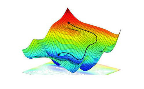
The process of searching for a minimum in the function J(w,b,X,ytrue) starts at an arbitrary point in the space determined by the initial parameters. At each iteration, the weights are updated, with the objective of approaching a point that reduces the error value. This process is known as gradient descent and is one of the most widely used optimisation techniques since it can be applied in most learning algorithms.

When a stochastic system or process is available (i.e. the system or process is connected to a random probability, in this case determined by the different observations in the sample), the so-called Stochastic Gradient Descent (SGD) method can be used, where samples are randomly selected instead of the whole data set for each iteration.

Other types of gradient descent, such as Batch Gradient Descent or Mini-batch Gradient Descent try to correct for the regularity of the oscillations by computing the cost function and weight updates, which provides robustness to the estimator and more direct paths to minima.

The adjustment of the weights in each iteration will be determined by the slope/derivative at the evaluated point and a multiplicative factor of this slope, which is introduced as a hyperparameter of the model known as the learning rate.

The SGD method is the simplest and most general method that can be used to update the network parameters. However, a multitude of optimisation algorithms have been proposed that exploit different characteristics of the types of spaces generated by artificial neural networks, and therefore improve the speed, efficiency and convergence of the training (such as AdaGrad, RMSprop, AdaDelta, Adam, etc.).

Initialisation of parameters

The performance of a neural network depends a lot on how its parameters are initialised when it starts training: if this is done randomly for each run, it is likely to be non-reproducible or not perform well. On the other hand, if constant values are used, it may take too long to converge. The initialisation will determine the starting point over the space of the error function, so it is relevant to adapt the values of the initial weights to the characteristics of the space in order to start from areas whose gradients are as close as possible to areas of high convexity.

The most frequent techniques for initialising weights are zero initialisation, random initialisation, Xavier initialisation (tries to avoid exponentially decreasing or increasing input signal magnitudes caused by gradient composition), or He initialisation (which pursues the same goal as Xavier initialisation, however, this method shows better performance with some activation functions).

Overfitting

One of the problems in training neural networks is the so-called overfitting: instead of learning a general map from inputs to outputs, the model may learn specific input examples and their associated outputs. This will result in a model that performs well on the training data set and poorly on new data due to a memorisation effect, with no generalisation capacity. To avoid this problem, some techniques can be applied to limit the capacity of the model without losing predictive power. The most commonly used techniques include the following:

• Gaussian noise: Introducing noise into the input of a neural network can be considered a form of data augmentation, as it increases the apparent number of different observations in the network. Therefore, adding noise to the input data of a neural network during training can, in some circumstances, lead to significant improvements in generalisation performance. Adding noise means that the network is less able to memorise the training samples because they are continuously changing, resulting in smaller network parameters and a more robust network that has a lower generalisation error.
• L2 regularisation: often referred to as weight decay, as it makes the weights smaller. It is also known as ridge regression and is a technique in which the sum of the squared parameters, or weights of a model (multiplied by some coefficient) is added to the loss function as a penalty term that must also be minimised.
• L1 regularisation: called Lasso Regression (Least Absolute Shrinkage and Selection Operator), it adds the "absolute value of the magnitude" of the coefficient as a penalty term to the loss function.
• Dropout: This is a probabilistic neuron elimination technique. During training, a certain number of layer outputs are randomly ignored, or "dropped out". This has the effect of causing the layer to be treated as a layer with a different number of nodes and therefore different connectivity to the previous layer. Each update of a layer during training is done with a different "view" of the configured layer.

Neural network architectures

This section aims to give an overview of some of the most common neural network structures, from the most basic one (the multilayer perceptron) to more complex neural networks: autoencoders, as an extension of the perceptron, recurrent neural networks, and convolutional networks.

Multi-layer perceptron neural networks

First, it is useful to analyse the minimum unit that makes up this type of neural network: the perceptron. This structure has an input data set, and an output neuron.

Inputs to the perceptron have a linear, unidirectional flow: inputs are connected directly to outputs through a series of weightings. This type of architecture is called feedforward, because the connections between the units do not form a cycle. Intuitively, this structure is analogous to a regression: each variable has an associated weight and the sum of all of them results in an output, which may be associated with an output function.
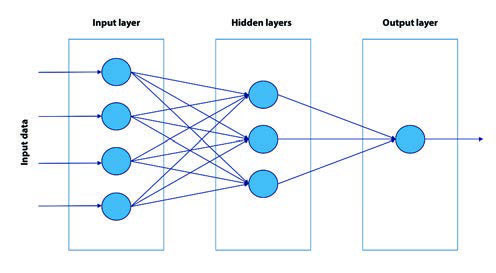
This structure can be extended to multiple layers with multiple neurons in each layer, resulting in multilayer perceptron neural networks.

Adding more complexity to the network by adding hidden layers increases its predictive power in non-linear problems. This enables neural networks to solve much more complex problems and compete with other advanced models. However, the extension of the architecture and the consequent increase in predictive power are associated with an increase in computational cost.

A special case can be considered when the activation function is the function ReLU(x) = max(0,x), the so-called of ReLU networks. These networks have special characteristics (they are easier to interpret, since this type of networks are piecewise linear continuous functions).

Autoencoders

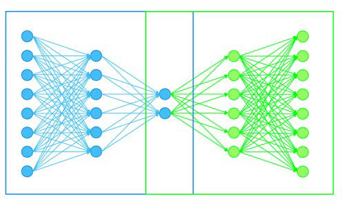
An autoencoder works analogously to a multilayer perceptron neural network, although the distribution of neurons in the hidden layers and the output layer are organised differently. The network is organised into an encoder, a common part and a decoder.

In simplified form, the network aims to establish a relationship between two sets through a biunivocal transformation (a bijective function). This is achieved by applying intermediate layers with a smaller number of neurons. Visually, the encoder can be understood as a data funnel that is responsible for reducing the input information into the output set. This final grouping of the encoder will be the initial input data of the decoder, which will be in charge, through the intermediate layers, of reconstructing the initial data.

This type of network can be used to reduce the dimensionality of a given generic data set, in noise removal, anomaly detection, encryption of information, etc.

Recurrent Neural Networks (RNN)

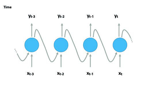
These networks are based on an architecture that allows the processing of temporal data, through the persistence of information over time. RNN consider time as a variable that modifies a given entity. This fact makes this type of architecture really useful to obtain interesting characteristics of sequential data.

Each neuron has two inputs: the initial input for each time unit and the output of the adjacent neuron. The existence of these cycles in the neurons allows the persistence of information from previous states. This information can be used to define future steps.

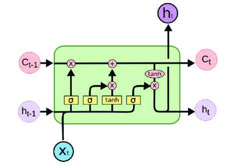
One of the classic architectures of this type of RNN is the LSTM (long short-term memory), which has the ability to maintain long-term memory. This algorithm has a "gate" that discards persistent information that is no longer useful for defining future steps. These gates are trained to detect which data are important in the sequence and should therefore be retained, and which should be discarded. Subsequently, related information can be passed along the long chain sequence for prediction.

Thanks to the long-term memory feature, this architecture is particularly useful for use in text understanding or time series prediction. While there are methods that also perform this function, these algorithms have the advantage of incorporating context and word order as predictive information.

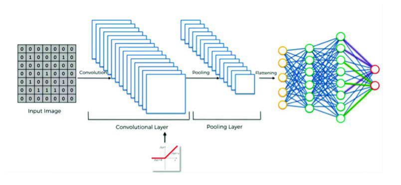
Convolutional networks

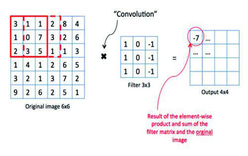
One of the architectures that play a fundamental role in computer vision are convolutional networks. In the case of image processing, the input data have a completely different format: they are pixels of an image, which are distributed three-dimensionally due to the three RGB channels (red, green and blue). In contrast to tabular data, they are considered spatial data due to the fact that a pixel is a magnitude of a point in a scene. Two neighbouring pixels correspond to neighbouring points in a scene, so they will have similar values.

The architecture is a variation of a multilayer perceptron that introduces convolutional layers. In the first convolutional layer, each neuron has an associated enclosure in the image, a function f. This function overlaps with adjacent frames of neurons belonging to the first convolutional layer, i.e. a function g. This overlapping is exploited by the convolution operator to obtain a function h = f * g which in a way summarises the information provided with the image. These regions considered are of constant dimension for each neuron.

Deep Learning Frameworks

Building neural network architectures from scratch can be a tedious job. Therefore nowadays there are a variety of frameworks that allow the development of Deep Learning models quicker and easier, without having to enter into the details of the underlying algorithm.

These deep learning frameworks provide pre-designed and optimised components to design, train and validate models through a high-level programming interface. Maintaining a framework is not an easy task (in fact, some of them are not maintained by their developers). It is therefore recommended that, when selecting a Deep Learning framework, priority should be given to those that are under active development.

• Tensorflow: this is one of the most popular Deep Learning frameworks thanks to its power and ease of use, offering various levels of abstraction in the creation and training of models. It is compatible with a wide variety of programming languages, with Python being the most widely used language. It is worth noting that the release of Tensorflow 2.0 has included numerous changes to improve productivity, simplicity and ease of use. 
• Keras: is an open source library written in Python that was created with the aim of providing rapid experimentation with neural networks, and can be run on various Deep Learning frameworks. It is characterised by its simplicity and straightforwardness, which is why it is considered a very good alternative for getting started in Deep Learning.
• PyTorch: a Deep Learning framework that has gained great mportance in recent years, especially in academia, becoming Tensorflow's main competitor. Pytorch was designed with the aim of accelerating the entire pipeline, from prototyping to production deployment, promoting scalable distributed training and performance optimisation. 
• MXNet: It is a flexible, scalable and fast Deep Learning framework, which has support in multiple programming languages, highlighting its distributed training functionality. However, compared to the previous frameworks, its popularity is lower.

These Deep Learning frameworks are commonly used in both research and production environments. Moreover, in line with the popularity acquired by cloud computing, it is common to use them in cloud environments, as they allow to take advantage of the benefits they offer: availability of major advances in terms of technological infrastructure (GPUs, TPUs, etc.), scalability, or cost reduction, among others.

Challenges and opportunities of integrating neural networks

Deep learning algorithms represent a promising field of research for automated pattern extraction in complex data. These algorithms develop a hierarchical architecture in layers of learning and data representation, where higher-level (more abstract) features are defined in terms of lower-level (less abstract) features. Deep learning solutions have yielded outstanding results in different applications, such as speech recognition, computer vision, image processing or natural language processing.

Despite the promising results obtained with the use of Deep Learning, there are still a number of challenges faced by the scientific community, companies and individuals using this technology:

• Data volume: In fully connected multilayer networks it is necessary to correctly estimate a high volume of network parameters (sometimes in the order of millions). The basis for achieving this goal is to have a large amount of data. However, collecting such a large set of annotated cases (cases where an identifying label has been defined, on which learning is performed) is, in many cases, a complex task. Different approaches have been used to solve this problem, consisting of both artificially increasing the volume of data and improving estimation methodologies, or a combination of both (e.g. data augmentation, sparse annotation, transfer learning, Patch-Wise Training or Weakly Supervised Learning).
• Data quality: Data sparsity, redundancy and null values or unbalanced datasets are information quality challenges in modelling processes. In the case of unbalanced datasets, the anomalous (minority) class is often the class to be learned (e.g. in the field of fraud detection, the minority class is precisely the presence of fraud). Training a network with this data often leads to the trained network being biased and may fall into the local minima of the cost function. Several methods can be used to improve data quality, including data cleaning, data normalisation, feature selection, or dimensionality reduction, among others.
• Temporality and non-static data: In multiple knowledge domains (such as medical, financial or manufacturing) there is a need to analyse evolution over time. Designing deep learning approaches that can handle temporal data is an important aspect that will require the development of novel solutions.
• Overfitting and time required for model training: these challenges stem from the need to use large volumes of data. Therefore, any solution that can increase the size of the data can also help solve the overfitting problem. Also, reducing learning time and achieving faster convergence are the focus of multiple studies.
• Interpretability: In many sectors and fields of knowledge (such as finance) it is important to understand what factors underlie a classification. Achieving interpretability is crucial to build trust and confidence and to encourage the use of decision support tools based on such models.

All these challenges, however, present opportunities and possibilities for future development and research: 
 

• Data enrichment: in order to train models, it is necessary to increase not only the number of individuals from which to extract features but also the number of features themselves. The current development of technology has made it possible to store heterogeneous data sources that have to be integrated and exploited. A possible solution could not only integrate the data and train a model, but also try to expand the number of layers, where each layer is trained on data from different sources (demographics, social networks, behaviour, etc.). 
• Federated data analysis and swarm learning: each organisation stores, exploits and manages its own databases. In many sectors, the use and integration of multiple databases from different organisations could provide better model training results. However, such training would have to be done without leaking sensitive information between organisations. Federated learning architectures and swarm learning allow training network models in a federated environment, including an additional security layer based on blockchain technology. 
• Model privacy: finally, privacy is an important concern, especially in environments where predictive models are deployed as a cloud service. There are lines of research aimed at eliminating vulnerabilities in this type of service.

Conclusions

Deep learning has been widely applied to problems such as computer vision, natural language processing and audiovisual recognition. In addition, the proliferation of startups and new technology service companies has led to the incorporation of the use of deep learning in multiple sectors, such as financial services with the emergence and development of Fintech.

One of the challenges facing the development of this type of model is the processing of non-static data, which is common in sectors such as finance. Although there is still a long way to go in implementing Deep Learning models in many sectors, this type of algorithm can probably improve customer knowledge, product recommendation, service improvement, process efficiency, or capital structure management, which would lead to maximising the value of corporations.

Therefore, further research is needed to address the various challenges that arise in different sectors in relation to the development of tools and platforms that include the techniques analysed for the implementation of Deep Learning models. 

The "Deep Learning​​" newsletter is now available for download on the Chair's website in both in spanish and english.​​